
Lyft Perception Challenge
Published:
Achieve pixel-wise identification of objects in camera images. It was hosted by Udacity and Lyft’s Level 5 Engineering Center. details https://www.udacity.com/lyft-challenge
github repo https://github.com/gwwang16/Lyft-Perception-Challenge
Overview
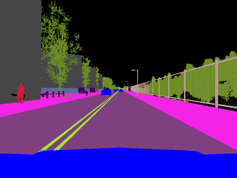
The goal in this challenge is pixel-wise identification of objects in camera images. In other words, the task is to identify exactly what is in each pixel of an image! More specifically, you’ll be identifying cars and the drivable area of the road. The images below are a simulated camera image on the left and a label image on the right, where each different type of object in the image corresponds to a different color.
The challenge time is from May 1st 10:00 am PST to June 3rd at 6:00 pm PST.
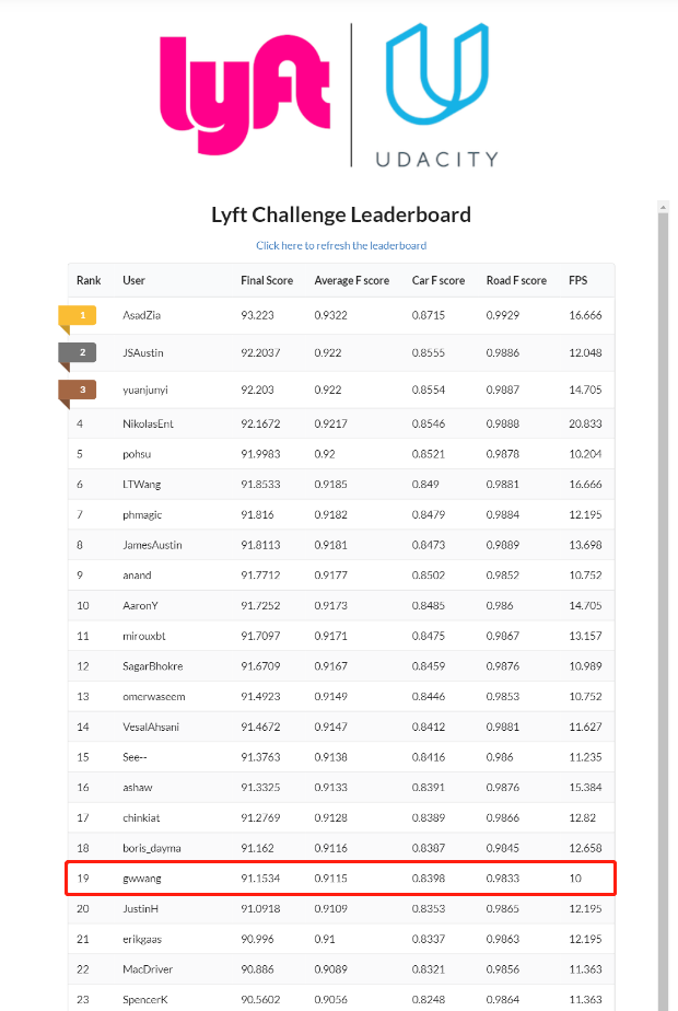
Result
I got the rank 19th finally.
The top 25 (only with U.S. work authorization) will be eligible for an interview with Lyft. So, I participated this challenge just for the fun of it.
The Data
The challenge data is being produced by the CARLA Simulator, an open source autonomous vehicle platform for the testing and derivative of autonomous algorithms. You can download the data here.
The dataset consists of images and the corresponding ground truth pixel-wise labels for each image.
The images and ground truth are both 3 channel RGB images and the labels for the ground truth are stored as integer values in the red channel of each ground truth image. The integer values for each pixel in the ground truth images correspond to which category of object appears in that pixel, according to this table:
| Value | Tag | Color |
|---|---|---|
| 0 | None | [0, 0, 0] |
| 1 | Buildings | [70, 70, 70] |
| 2 | Fences | [190, 153, 153] |
| 3 | Other | [72, 0, 90] |
| 4 | Pedestrians | [220, 20, 60] |
| 5 | Poles | [153, 153, 153] |
| 6 | RoadLines | [157, 234, 50] |
| 7 | Roads | [128, 64, 128] |
| 8 | Sidewalks | [244, 35, 232] |
| 9 | Vegetation | [107, 142, 35] |
| 10 | Vehicles | [0, 0, 255] |
| 11 | Walls | [102, 102, 156] |
| 12 | TrafficSigns | [220, 220, 0] |
Given that the values are small (0 through 12), the 3-channel label images appear black at first glance. But if you plot up just the red channel (label_image[:,:,0]) you’ll see the labels, like this:
| Camera Image | 3-Channel Label Image | Label Image Red Channel |
|---|---|---|
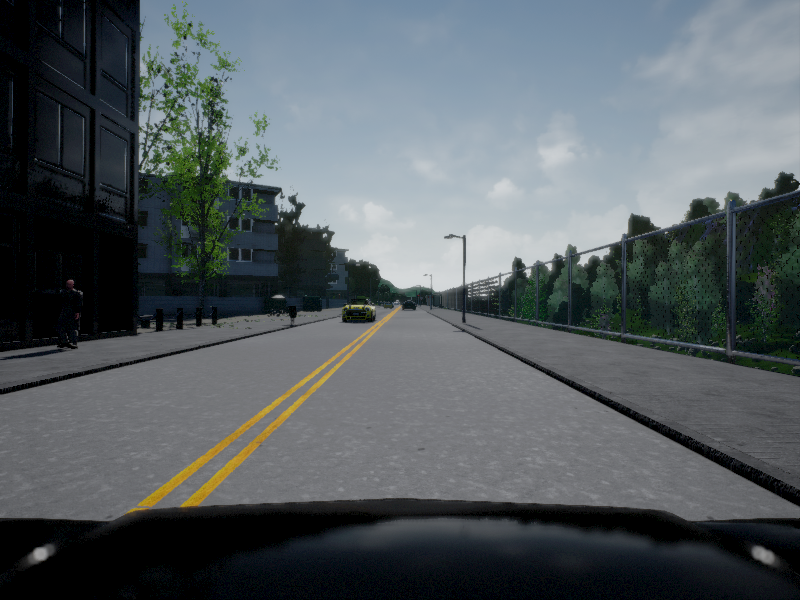 |  |  |
The task is to write an algorithm to take an image like the one on the left and generate a labeled image like the one on the right. Except you will be generating a binary labeled image for vehicles and a binary labeled image for the drivable surface of the road. You can ignore other things like trees, pedestrians, etc.
Your solution will be run against a hidden test dataset. This test set consists of images that are different from the training dataset, but taken under the same environmental conditions. Your algorithm will be evaluated on both speed and accuracy.
Weighted $F_\beta$Score
In some cases, you might be more concerned about false positives, like for example, when identifying where the drivable road surface is, you don’t want to accidentally label the sidewalk as drivable. In that case the precision of your measurement is more important than recall.
On the other hand, you might be more concerned with false negatives, for example, when identifying vehicles you want to make sure you know where the whole vehicle is, and overestimating is not necessarily a bad thing. In that case, recall is more important than precision.
In most cases, however, you would like to strike some balance between precision and recall and you can do so by introducing a factor β into your F score like this:
\[\rm{F}_\beta = (1+\beta^2)*\frac{\rm{precision}~*~\rm{recall}}{\beta^2*\rm{precision}+\rm{recall}}\]By setting β<1, you weight precision more heavily than recall. And setting β>1, you weight recall more heavily than precision.
For this challenge you’ll be scored with β=2 for vehicles and β=0.5 for road surface.
Your final F score will be the average of your\(\rm{F}_{0.5}\) score for road surface and your $\rm{F}_{2}$ score for vehicles.
β(vehicle)=2
β(road)=0.5
\[\rm{F_{avg}} = \frac{\rm{F}_{0.5} + \rm{F}_{2}}{2}\]Incorporating Frames Per Second (FPS)
The speed at which your algorithm is also important and will be factored into your final score. You’ll receive a penalty for running at less than 10 FPS:
\[\rm{Penalty_{\tiny{FPS}}} = (10-\rm{FPS}) > 0\]Here’s how your final score on the leaderboard will be calculated, incorporating both your F score and FPS:
\[\rm{Final~Score} = \rm{F_{avg}}*100 - \rm{Penalty_{\tiny{FPS}}}\]Model
fcn-mobilenet
…
Reference:
CARLA Simulator: https://github.com/carla-simulator/carla
MobileNets: Efficient Convolutional Neural Networks for Mobile Vision Applications :
https://arxiv.org/abs/1704.04861
https://github.com/keras-team/keras/blob/master/keras/applications/mobilenet.py
Keras implementation of Deeplab v3+ with pretrained weights: https://github.com/bonlime/keras-deeplab-v3-plus/blob/73aa7c38c4c8498ca0ddb831f1c7d744ca57daee/model.py
keras-mobile-colorizer: https://github.com/titu1994/keras-mobile-colorizer